Gromacs [1] is one of the most widely used software for molecular dynamics (MD) simulation of macromolecules. One of the previous articles, explains the installation of Gromacs on Ubuntu. This article is about the execution of Gromacs simulating a simple protein. This is a simple tutorial for MD simulation of a protein.
In this tutorial, we are going to simulate chain A of insulin (PDB ID: 1ZNI).
1. Preparing protein file
Remove the other chains and hetatoms including the water molecules (HOH) from the protein file. You can use an editor such as vim, notepad++ in Ubuntu and Windows. Hetatoms can also be removed by using the following command:
$ grep -v HETATM 1zni.pdb > 1zni_new.pdb
2. Converting PDB to gmx and generating topology
pdb2gmx module is used to generate the topology of proteins. Make sure the protein file consists of protein atoms only otherwise it will be giving errors.
$ gmx pdb2gmx -f 1zni_new.pdb -o 1zni_processed.gro -water spce
It will ask to select the force field that contains information to be written to the topology. This an important step, therefore, select an appropriate field relevant to your study. In this tutorial, we will be using the OPLS all-atom force field, so type 15 in the terminal. There are several other arguments that you can pass in pdb2gmx, type
$ gmx pdb2gmx -h
to know about these options.
Now, you have generated three new files: 1zni_processed.gro, posre.itp, and topol.top. 1zni.gro is a structure file formatted by GROMACS which contains all atoms defined in the force field, posre.itp file contains the information used to keep the non-hydrogen atoms in place by defining a constant, and topol.top file contains the system topology.
Remember to remove other chains from the pdb file before converting it to the gmx format. If you look into the topology file (Fig. 1), there will be different sections such as the first section shows the forcefield parameters used (here, OPLS all-atoms), [atoms] section defines all atoms present in the protein including their atom names, mass, and charge, subsequent sections include position restraint, water topology, [system], and [molecules] (Fig. 2).
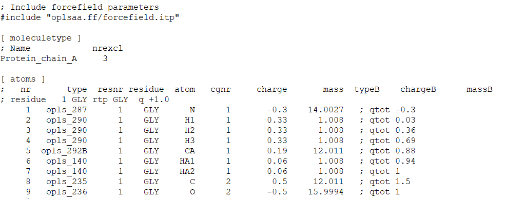
Fig. 1 A screenshot of topol.top file.

Fig. 2 Sections in topol.top file.
Since we have generated the topology file, we can move on to the next step.
3. Defining box
To build a system, we need to define a box of proper dimensions for the protein. You can choose different types of boxes but here we will be using a rhombic dodecahedron box as it can save the number of water molecules during the solvation of protein (discussed in the next step). editconf module will be used for defining the box.
$ gmx editconf -f 1zni_processed.gro -o 1zni_box.gro -c -d 2.0 -bt dodecahedron
here, -f defines the input filename, -o is the output file, -c is used to keep the protein in the center inside the box, -d defines the distance of the protein from the box edges (which should be at least 1.0 nm to avoid the periodic images of protein otherwise, the forces could be miscalculated), and -bt is the type of box.
Now, we have successfully defined the box around the protein. Let’s move on to the next step.
4. Solvating the protein
Now, we will fill the box with water using the solvate module which keeps track of the newly added water molecules and writes to the topology file.
$ gmx solvate -cp 1zni_box.gro -cs spc216.gro -o 1zni_solvate.gro -p topol.top
here, -cp defines the protein configuration obtained in the last step, -cs is the solvent configuration which is a part of GROMACS, -o defines the name of the output file, and -p is the topology file.
Now, if you open the topol.top file, you will find SOL molecules at the end of the file as shown in Fig. 3. The topology file will not be updated in case a non-water solvent is used.
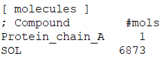
Fig. 3 SOL molecules added after solvation.
5. Adding ions
Now, we need to add ions to the charged protein by using the genion module. It requires a grompp module to produce a .tpr file which is used as an input to the genion command. First, we need an MD parameter (.mdp) file which contains all the coordinates and topology information to generate a .tpr file. The ions.mdp file can be downloaded from here.
As you can see in ions.mdp file, we have defined the periodic boundary conditions (PBC) which are used to minimize edge effects in a finite system, so that there are no boundaries in the system. The artifact caused by the boundaries is now replaced by the PBCs [2]. After that you can see, the verlet cut-off scheme has been preferred over the groups of atoms because it offers several advantages such as it works well for the systems where energy conservation is necessary and also works well on CPUs with SSE and AVX.
Let’s generate .tpr file and then add ions.
$ gmx grompp -f ions.mdp -c 1zni_solvate.gro -p topol.top -o ions.tpr
$ gmx genion -s ions.tpr -o 1zni_solvate_ions.gro -p topol.top -neutral
It will prompt you to select a group of solvent molecules and choose “Group 13- SOL” to embed ions.
In the genion command, -s defines the structure file as input, -o defines the output file, -p is the topology file, and -neutral is defined to add only the necessary ions to neutralize the net charge on the protein. If you look at the terminal, it would be showing you the exact number of ions added whether positive or negative. That’s because if you check the very first topol.top file and look at the [atoms] section at the last line, it would be showing the total charge on the protein as “qtot -2”. In this case, it is -2, therefore, it has added 2 NA ions and 0 CL ions to neutralize the protein.
Now, if you look again into the topol.top file under the [molecules] directive, it would be showing the number of ions added as shown in Fig. 4.

Fig. 4 Number of ions added to the protein.
After adding ions, let’s move on to the next step of energy minimization.
6. Energy minimization
Energy minimization is used to stabilize the structure and make sure it does not have any steric clashes. For this, another input parameter file is required, which can be downloaded from here. First, using the grompp command, we will generate a binary input file, .tpr which contains simulation, structure, and topology parameters.
$ gmx grompp -f em.mdp -c 1zni_solvate_ions.gro -p topol.top -o em.tpr
Now, run the energy minimization using mdrun.
$ gmx mdrun -v -deffnm em
It would take a few minutes to finish. In order to know, whether the energy minimization was run successfully, the potential energy must be negative (in this case, Epot is –3.5583712e+05) and Fmax must be less than 1000 KJ/mol/nm which was set as the maximum force in em.mdp file. After finishing mdrun, it would look like this:
Steepest Descents converged to Fmax < 1000 in 389 steps

Potential Energy = -3.5583712e+05

Maximum force = 8.7233093e+02 on atom 55

Norm of force = 3.6632029e+01
If the Fmax is greater than that then increase the nsteps for minimization or check the emstep and emtol.
You can also plot the graph for the Epot using em.edr file as follows. Make sure you have installed xmgrace on your system. If not then type $ sudo apt-get install grace.
$ gmx energy -f em.edr -o potential.xvg
It will prompt you to select and type “10 0”. The graph is shown in Fig. 5.

Fig. 5 A graph of potential energy vs the number of steps in energy minimization.
Now that our system at minimum energy, we can move on to the next step.
7. Equilibration
Before running MD, we need to equilibrate the ions and the solvent around the protein and bring the system at a particular temperature at which we want to simulate. After bringing it to a particular temperature, constant pressure is applied to bring it to a proper density. Equilibration is done in two phases: isothermal/isochoric and isobaric.
i) Phase-I
It is conducted under a constant number of particles, volume, and temperature (NVT ensemble). We will be using another input file, nvt.mdp that can be downloaded from here. The timeframe provided for NVT should bring the temperature of the system to reach a plateau at the desired value. Generally, 100 ps are enough which we will be using here and the temperature will be 300 K. First, we will use the grompp command and then mdrun for NVT.
$ gmx grompp -f nvt.mdp -c em.gro -r em.gro -p topol.top -o nvt.tpr
$ gmx mdrun -v -deffnm nvt
This step may take a while to finish depending on the machine you are using. After the job is finished, you can see the temperature progression by using the following command:
$ gmx energy -f nvt.edr -o temperature.xvg
On the prompt, type “16 0” to select the temperature of the system and exit respectively. The plot will look like as shown in Fig. 6. As you can see from the graph, the temperature of the system has reached a set value of 300 K and remains stable for equilibration. After that, we can proceed toward the next phase of equilibration.

Fig. 6 A graph showing the temperature of the system under the NVT ensemble.
ii) Phase-II
After stabilizing the temperature, we should now stabilize the pressure of the system by keeping the number of particles, pressure, and temperature constant (NPT ensemble). We will use a 100 ps timeframe for this phase as well. The npt.mdp file can be downloaded from here. If you look into the npt.mdp file under “Bond parameters”, the “continuation” is set to “yes”, because the simulation is in continuation from Phase-I.
Grompp and mdrun modules will be used in this phase also.
$ gmx grompp -f npt.mdp -c nvt.gro -r nvt.gro -t nvt.cpt -p topol.top -o npt.tpr
$ gmx mdrun -v -deffnm npt
This step may also take a while to finish depending on the machine you are using. After the job is finished, you can see the pressure progression by using the following command:
$ gmx energy -f npt.edr -o pressure.xvg
On prompt, type “18 0” to select the pressure of the system and exit respectively. The graph is shown in Fig. 7 and the moving average is shown in the red dotted line.
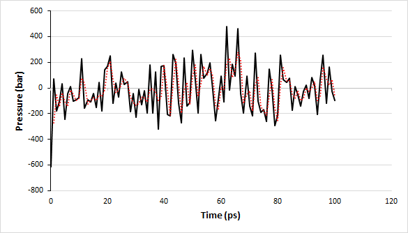
Fig. 7 A graph showing the pressure values over the time period of 100 ps under the NPT ensemble.
The pressure values fluctuate over time as evident from the graph, therefore, it is quite difficult to differentiate the obtained values from the reference value (i.e., 1 bar). Let’s plot a graph for density.
$ gmx energy -f npt.edr -o density.xvg
When prompted, type “24 0” for density and exit. The density graph is shown in Fig. 8 and the moving average is shown in the red dotted line.

Fig. 8 A graph showing the density values over the time period of 100 ps.
The calculated average value of density over a time period of 100 ps is 1003.617 kg/m3 which is very close to the experimental value of 1000 kg/m3 and also very close to the expected density of SPC/E model 1008 kg/m3. The density values are very stable and therefore, the system is well equilibrated with respect to the pressure and density.
Now that we have a stable system, we can move on to the last step of MD.
8. Running MD
We will need an input file md.mdp which can be downloaded from here. We will run a 1 ns MD simulation which is just for the purpose of demonstration otherwise, optimally, 30 ns or 50/60 ns MD simulation is done. 30 ns should be enough but if RMSD is not a straight line then increase the duration of the MD run. Currently, 100ns is the most widely accepted.
If you look into the md.mdp file, you will see the
nsteps = 500000
which is equal to 1000 ps = 1 ns.
The way to determine the nsteps for MD is explained below:
Let’s assume time in ns is x and 1000 ps = 1 ns, therefore, the general equation will be:
nsteps * timestep (ps/step) = 1000 * x ps = x ns
So, if you want to run MD for 1 ns, then the equation will be,
500000 (nsteps) * 0.002 time (ps/step) = 1 ns ###The timestep in production MD runs (dT) is 2 fs (i.e., 0.002 ps).
For more details on nsteps calculation, read this article.
First, we will generate the .tpr file using grompp and then run production MD.
$ gmx grompp -f md.mdp -c npt.gro -t npt.cpt -p topol.top -o md_0_1.tpr
$ gmx mdrun -v -deffnm md_0_1
Since MD run takes a long time to finish, therefore, you would like to run for which you can use the nohup command as shown below:
$ nohup gmx mdrun-v -deffnm md_0_1 -cpi md_0_1ms.cpt -nb gpu
You can check the status by using the command $ jobs or $ top.
If you want to rerun or extend an MD simulation run, then use the -cpi and -append options in the mdrun command.
This ends the MD simulation tutorial, and the MD result analysis will be explained in the upcoming article. If you have any queries, email muniba@bioinformaticsreview.com.
References
- Abraham, M. J., Murtola, T., Schulz, R., Páll, S., Smith, J. C., Hess, B., & Lindahl, E. (2015). GROMACS: High performance molecular simulations through multi-level parallelism from laptops to supercomputers. SoftwareX, 1, 19-25.
- Abraham, M. J., Van Der Spoel, D., Lindahl, E., & Hess, B. (2015). the GROMACS Development Team (2014) GROMACS User Manual Version 5.0. 4.