Structure modeling of chemical compounds finds essential application in the field of cheminformatics. It is used to study the structural stability, metal-ion bonding, the presence of electrons, closed and open shell energies, the reactivity of complexes, molecular orbital analyzes, molecular mechanics, and so on. There is some software available for structural modeling of chemical compounds/complexes and the most widely used are Gaussian [1] and ORCA [2].
Gaussian software allows users to study molecular mechanics, ground-state semi-empirical calculations, Density functional theory (DFT), wave-function stability analysis (HT and DFT), electronic correlation, geometric optimization, vibrational frequency analysis, and so on.
In this tutorial, we will discuss Gaussian (G09) software and its application to perform molecular orbital analysis of a compound. This basic analysis requires an input file generated either using G09 or Avogadro. However, this tutorial will cover both the options and then finally the job will be run on G09 providing a detailed profile of orbitals in a compound/complex.
Let’s prepare the input file first.
1. Preparing the input file
The input file for the analysis can be generated by Gaussian itself but the coordinates need to be calculated and input manually, therefore, it’s easier to generate input file using Avogadro or ChemDraw and then open in Gaussian for further analysis. We will go through the steps for input file generation using both the software one by one.
i) using Avogadro
- Draw molecule.
- Go to ‘Extensions’ –> ‘Optimize Geometry’
- Go to ‘Extensions’ –> ‘Gaussian…’
- A window will appear as shown in Fig. 1, select the appropriate options as per your requirements. Our calculation is ‘Geometry Optimization’ and the other default parameters. After that, click ‘Generate’ and save the file as Gaussian Input Deck (.com) in the same folder.
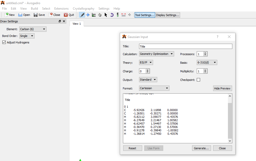
Fig. 1 A screenshot showing the parameters of input file generation in Avogadro.
ii) using ChemDraw
- Draw molecule.
- Go to ‘Calculation’ –> ‘MM2’ (to optimize the geometry)
- Save the file as a .gjf file.
2. Running the job in Gaussian (G09)
- Open the G09.
- Go to ‘File’ –> ‘Open’. Open the .com/.gjf file generated using ChemDraw/ Avogadro.
- A new window will appear showing different sections (Fig. 2).

Fig. 2 A screenshot of Gaussian displaying different sections for job submission.
The first line is the path of the file.
“%Section” specifies the name of checkpoint file.
“Route Section” is the main job defining section, where you can define which test you want to run. For this purpose, a specific keyword is used along with the command “Pop” explained as follows:
"Pop" = "Reg" # displays HOMO-5 up to LUMO+5 orbital information
"Pop" = "Full" # displays information of all orbitals
"Pop" = "NBO" # for Natural Bond Order analysis
"Pop" = "None" # no orbital information is displayed
"Pop" = "MK, CHELP, OR CHELPG" # produce charges fit to electrostatic potential (ESP)
“Title Section” allows the user to enter a job name.
“Charge, Multipl.” allows specifying the charge and spin multiplicity of the molecule separated by a space.
“Molecule specification” displays the atoms and their coordinates. These coordinates are calculated by Avogadro or ChemDraw else the user needs to calculate them manually.
That was about the input parameters, you can change them as per your requirements. Now, let’s get back to our job submission.
- Since we want molecular orbital analysis including the d-orbitals, therefore, we will use
Pop=Fullcommand. So, type the following in the Route Section:
Pop=Full FormCheck and click on ‘OK’ box present on the right side.
As you can see, another command FormCheck has been added. This command is used to create a file which contains the information of all molecular orbitals and can be plotted later.
- The memory is allocated suitably depending upon the configuration of your workstation.
- You can see the progress in the ‘Run Progress’ bar, it will be changed to ‘Ready to run processing start’.
- Now, to execute the g09 command, either click on
 or go to ‘Process’ –> ‘Begin Processing’.
 - After that, it will prompt for the folder where you want to save your output file. Click ‘Save’.
- Again, you will notice that the Run progress bar has changed the status to ‘C:\G09W\l1 is executing’.
This job takes a long time to finish, wait until it finishes providing the output files. These files can then be used to visualize the d-orbitals. The analyzes of output results will be explained in the upcoming articles.
References
- Frisch, M. J., Trucks, G. W., Schlegel, H. B., Scuseria, G. E., Robb, M. A., Cheeseman, J. R., … & Nakatsuji, H. (2009). Gaussian 09, revision A. 1. Gaussian Inc. Wallingford CT, 27, 34.
- Neese, F. (2012). The ORCA program system. Wiley Interdisciplinary Reviews: Computational Molecular Science, 2(1), 73-78.